ABSTRACT:
In this work we have studied energy flow in acoustic billiards, focusing on irregular billiards with and without current effects. The open systems were modeled with an imaginary potential as a source and drain. We have used the finite difference method to model the billiards. General features of the systems are reported and effects of the measuring probe on the wave function are discussed.
THEORY
Billiards in general:
In this chapter we will present the foundations of billiards and chaos
Classical chaos and billiards
This work will focus on three types of two-dimensional billiards. Theoretically a billiard is a perfect billiard table on which a ball bounces from wall to wall without experiencing any friction or other energy loss. In this work we study acoustic waves instead of particles, but the equations are still the same. Analytical expressions for the wave functions and eigenvalues may be derived if the billiard is, for example,rectangular.
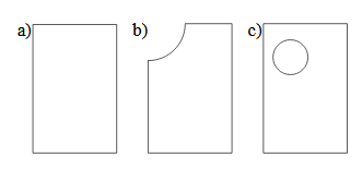
Three Different Types of Billiards; (a) Rectangular Billiard (B) Sinai Billiard With Broken Corner (C) Sinai Billiard With Internal Hole.
MODELLING
In this chapter we present the billiards that we modeled and we also show how they may be implemented. MatLab was used both in the calculations and for the visualisation. Since analytical expressions only exist for the rectangular billiard, all the calculations will be performed numerically.
Discretization:
The continuous system has to be discretized in order to make our numerical calculations. The two most common methods to do this are the finite difference method (FDM) and the finite element method(FEM). The FDM is very easy to understand and to implement, while FEM is harder. Why one would like to use FEM is because it gives faster calculations, although for this work we have chosen FDM because of its simplicity and numerical robustness.
Boundary conditions:
Boundary conditions (b.c.) are necessary in order to model our systems. Assume a surface S with a boundary ∂S, and a value ψ(x,y) at the point (x,y) on S. There exist two kinds of b.c. we may use, one is the Dirichlet b.c. which tells that the function should have a certain value at the boundary, most often zero. In this work we will use another type of b.c., the Neumann b.c., which instead tells that the normal derivative of the function should be zero at the boundary.
Solving the matrix:
The FDM together with the Neumann b.c. gives a penta-diagonal matrix, see figure 3.2. The matrix represents the operator ∇2, and can be of three different types depending on which of of the Sinai billiards that is managed. Solving the eigenvalue problem ∇2ψmn = −k2mnψmngives the solution where we can extract the frequency for the system for the eigenstate mn from k2 mn, and ψmn is the wave function for that particular eigentstate. Because of its convenience in handling matrices, MatLab was a natural choice to solve this eigenvalue problem.
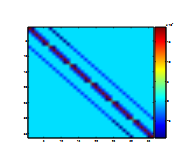
6×6 Point-system Matrix With Neumann Boundary Conditions Representing the Rectangular Billiard.
RESULTS
In this chapter we present the results of the calculations for the three billiards: a) a rectangular billiard; b) a Sinai billiard with broken corner; c) a Sinai billiard with an internal hole. The first section contains general results about the model itself.
General results:
In this section we present some general results for the model itself, i.e. tests with the rectangular billiard, for which there are analytical expressions with which we can compare our results.
Closed billiards:
First of all we want to examine our system in its normal state without any disturbance to be able to compare the changes when we add our potentials.
Rectangular billiard
In order to verify the numerical model used herein, we compare three example modes, figure 4.2, with corresponding analytical solutions, and conclude that they are in excellent agreement.
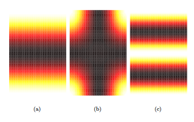
Three Low Modes of the Rectangular Billiard, Plotted as |ψ|2.
Open billiards:
In order to create an energy flow through the system we open up our billiards and study two cases, when there is one in- and one outflow and when there also exists a well, representing an antenna. Experiments have shown that the presence of antennas broaden and shifts the resonances somewhat, but this does not change the distributions in chaotic systems.
Statistics extracted from our models:
Acoustic resonators were studied by Schaadt where the same statistical properties as in this work were investigated. The statistics are only valid for modes in a certain class of symmetry. The procedure to isolate such a class is explored. Since this work mostly focuses on chaos effects we have chosen not to look at the symmetric billiard, but to only examine the two Sinai billiards. Thus this chapter will only present results for our Sinai billiards.
CONCLUSIONS
The objective of this work was to examine systems representing different kinds of billiards which includes imaginary potentials mimiking source, drain and an antenna. What we noted here was that the size of the antenna had to be fairly large, around 20% of the source and drain potentials, in order to give a visible disturbance on the energy flow. The tool used in these studies was based on finite difference approximations.
The electron cavity studied by Hakanen was modelled in a similar fashion to our systems. It also had a source and drain, and the equation used was the the quantum mechanical correspondence to Helmholz equation, the Schr ̈odinger equation.
Statistics show that the first Sinai billiard is of less chaotic nature than the second one. Histograms showing the spacings between eigene nergies imply that the distribution for the first Sinai billiard is affected by both chaotic and non-chaotic distribution while the second Sinai billiard is mostly governed by a chaotic distribution.
One conclusion of this chapter is that our Sinai billiards have GOE statistics. Experiments have already shown that the time-reversal process is stable and thus our result was expected.
FUTURE WORK
There are still interesting work to be done using the present model. One should improve the speed of the calculations so larger systems can be used. This would in turn allow higher frequencies to be included. This could be done by using a better eigenvalue solver for large systems.
In order to make comparison between our acoustic results and quantum theory more straight forward one could do the same analysis but in a system equivalent. This system has already been studied using both electrical circuits.
Conclusions and future work and using quantum theory. It would be interesting do study this both with and without an antenna. One last thing that would be interesting is to apply the Schr ̈odinger equationto the billiards in this work, yet another way to be able to perform analog studies between classical and quantum mechanical system.
Source: Linkopings University
Author: Lina F ̈alth
>> Antenna Analysis using Matlab for Engineering Students