ABSTRACT
The structure of an animal’s eye is determined by the tasks it must perform. While vertebrates rely on their two eyes for all visual functions, insects have evolved a wide range of specialized visual organs to support behaviors such as prey capture, predator evasion, mate pursuit, flight stabilization, and navigation. Compound eyes and ocelli constitute the vision forming and sensing mechanisms of some flying insects.
They provide signals useful for flight stabilization and navigation. In contrast to the well-studied compound eye, the ocelli, seen as the second visual system, sense fast luminance changes and allows for fast visual processing. Using a luminance-based sensor that mimics the insect ocelli and a camera-based motion detection system, frequency-domain characterization of an ocellar sensor and optic flow (due to rotational motion) are analyzed. Inspired by the insect neurons that make use of signals from both vision sensing mechanisms, complementary properties of ocellar and optic flow estimates are discussed.
BACKGROUND
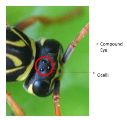
Figure 1: Insect Compound Eye and Ocelli
The compound eyes and ocelli are shown in Figure 1, head of a flying insect (Polistes). The structure of compound eyes (large, two on the sides) is seen in Figure 2. The compound eyes are composed of units called ommatidia. Each ommatidium unit functions as a separate visual receptor, consisting of a lens, cornea, a crystalline cone, light sensitive visual cells and pigment cells (Figure 3). There may be up to 30000 ommatidia in a single compound eye.
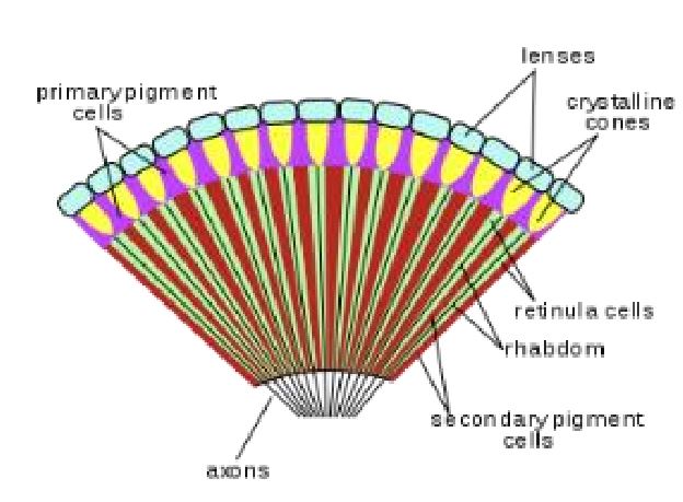
Figure 2: Structure of Compound Eye
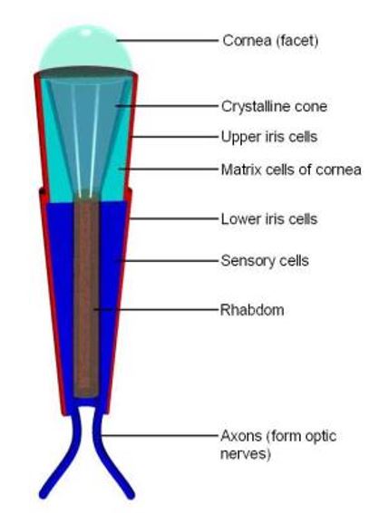
Figure 3: Structure of Ommatidium
Frequency Domain Characterization of an Ocellar Sensor and Optic Flow
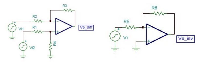
Figure 9: Subtractor and inverter: Subtractor is used for antagonistic subtraction of filtered signals
This stage includes a difference amplifier to subtract right-left filter outputs and front-back filter outputs. The difference amplifier output from the right-left inputs estimates the roll rate. The difference amplifier output from the front-back inputs is inverted (for sign change) by an inverting amplifier. Inverting amplifier output estimates the pitch rate (See the blocks in Figure 9).
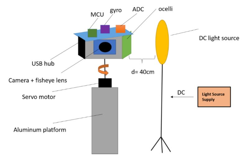
Figure 16: Illustration of Test Setup: Light source has its own DC supply to avoid issues of flickering
Illustration of Test Setup: Light source has its own DC supply to avoid issues of flickering. Information from camera, MCU, gyro, ADC are transferred to the host computer via a USB hub.
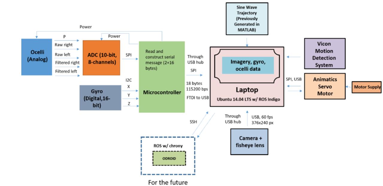
Figure 20: System block diagram: All the data collected is stored in laptop
The servo motor can be operated in either position or velocity mode. Velocity mode does not offer control in position. Motor is controlled by sending serial messages in Ani-Basic language. The command information and serial communication are specified. For both position and velocity modes, specific trajectory files are created in Matlab that include velocity/position trajectory (e.g. sine wave, square wave), and acceleration information.
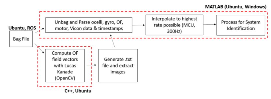
Figure 22: Post-processing block diagram: Optic flow vectors are computed and extracted as a text file
Post-processing block diagram: Optic flow vectors are computed and extracted as a text file. The bag file is parsed, interpolated and processed for data analysis.
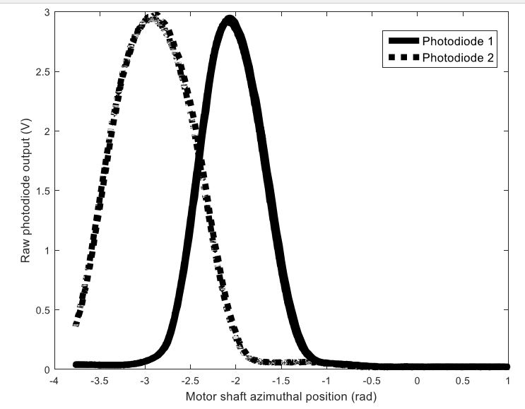
Figure 25: Bent photodiode output vs. motor shaft azimuthal position
Bent photodiode output vs. motor shaft azimuthal position: Photodiode field of views are partially overlapping, which is required for the ocellar sensor to work. In this (incorrect) configuration, there are angles where simulated roll motions do not produce any change in the photodiode outputs.
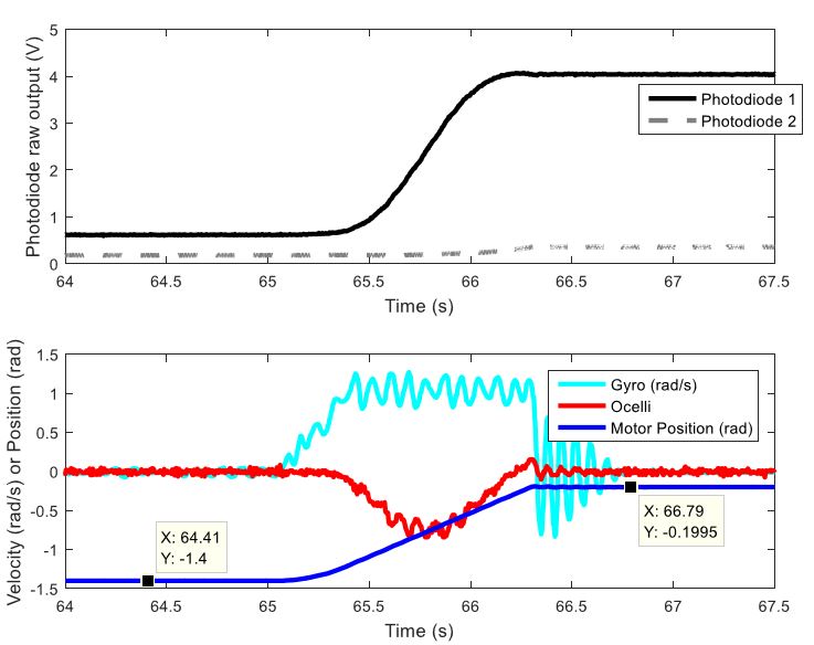
Figure 27: Ocelli in invalid range: (Above) Asymmetric photodiode raw output
Figure 27 shows an invalid region (azimuthal position changes from -1.4 to -0.2 radians). In this range, photodiode outputs are not symmetric to each other. Ocelli is not in agreement with gyro. Using this data, the maximum displacement for the ocellar circuit is determined to be 1 radian. All of the following characterizations are done in this valid region.
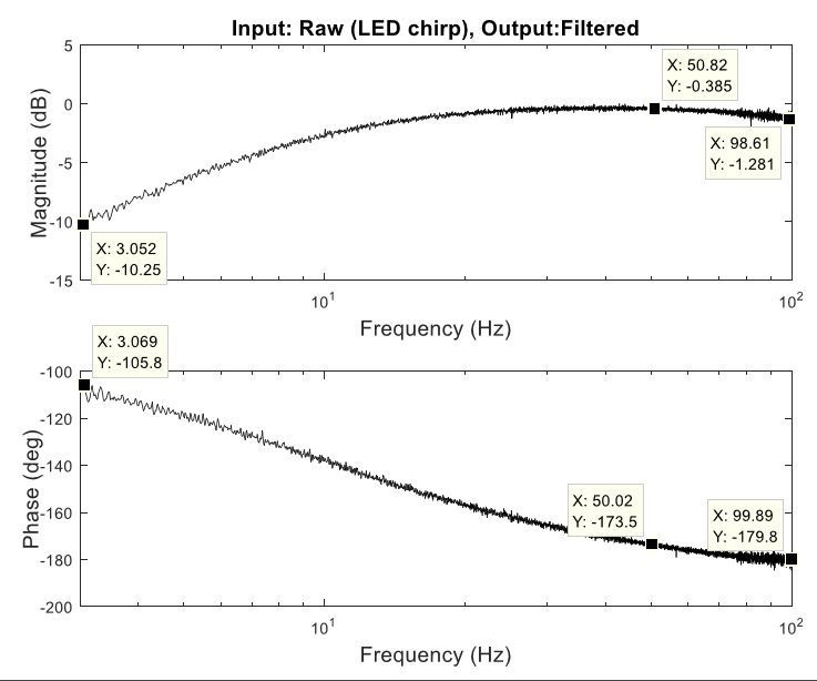
Figure 32: Right band-pass filter measured transfer characteristics in response to LED chirp
Figure 32 shows the frequency response of the circuit from the photodiode input from LED to the filtered output. The magnitude response starts from -10.25 dB and reaches to -0.29dB at 50 Hz. Then it decays to -1.281dB at 98.6 Hz. The phase response starts from -105.8 degrees at 3 Hz, decreasing to 180.5 degrees at 98.76 Hz.
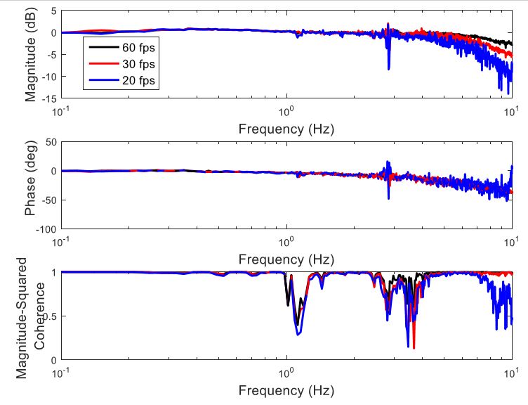
Figure 37: Optic flow frequency response with different frame rates
Optic flow frequency response with different frame rates, as seen by input gyro: As the frame rate decreases, roll-off at higher frequencies is steeper. Higher frame rate results in better coherence. Phase delay does not change due to frame rate.
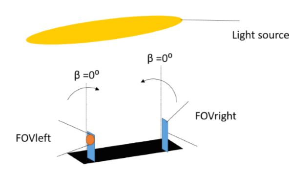
Figure 44: Bending illustration: The photodiodes should share an intersecting field-of-view (FOV)
Bending illustration: The photodiodes should share an intersecting field-of-view (FOV) towards the light source for the sensor to operate. Bending values 30⁰<β<45⁰ were observed to give symmetric photodiode outputs. β=90⁰ completely overlaps the field of views, without distinct horizons for each photodiode.
SENSOR FUSION
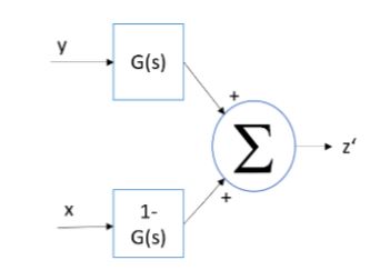
Figure 45: Illustration of complementary filter
Gyroscope is good for ‘short-term’, is known to have poor drift characteristics, however it is able to give fast response. An ideal combination would be a fast transient response with no drift, by combining good qualities from two measurements. Theoretically, if a time varying signal is applied to both a low-pass and high-pass filter with unity gain, the sum of the filtered signals should be identical to the input signal. (See Figure 45). Assume that x and y are noisy measurements of some signal z, x employing low-frequency noise and y employing high-frequency noise. z’ is the estimate of the signal z produced by the complementary filter.
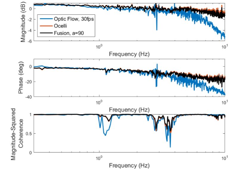
Figure 47: Frequency response ocelli , optic flow, and their weighted-average fusion: Ocelli and optic flow time domain signals are combined to obtain a result close to ocelli
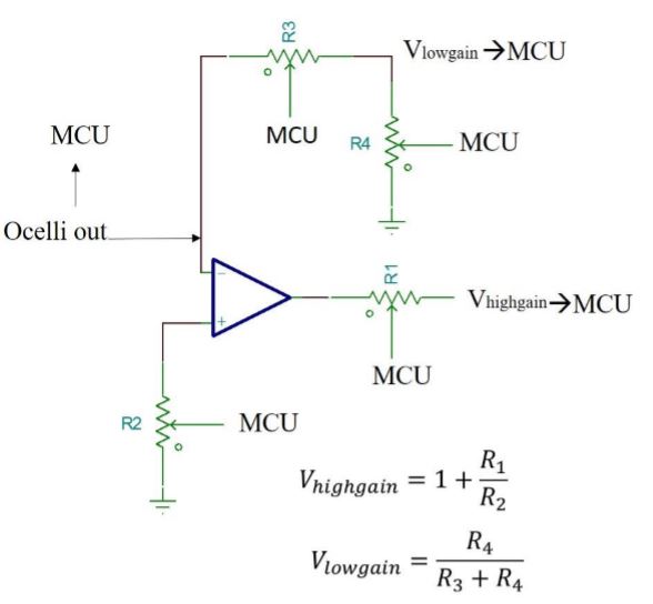
Figure 50: Ocelli gain adjustment approach: Gains>1 are tuned by non-inverting op-amp
Ocelli gain adjustment approach: Gains>1 are tuned by non-inverting op-amp. Gains
CONCLUSION AND FUTURE WORK
Conclusion
Frequency-domain characterization of optic flow and ocellar sensors are presented. The advantages and disadvantages for both sensing mechanisms are discussed. In summary:
- Ocellar sensor shows a relatively flat magnitude response and less phase delay than optic flow.
- Ocellar sensor is attractive for high-rate loop closure since it is cheaper and faster from high quality cameras.
- The displacement dynamic range of the ocellar sensor is observed to be 1 radian with this setup, due to the small size of the light source. Using a bigger light source, higher displacements may be achieved.
- The frequency dynamic range of ocellar sensor is observed to be up to 10 Hz with motion, and up to low-frequency cutoff without motion. 10 Hz is a limitation from mechanical test setup, higher motion frequencies are expected due to the circuit simulation and LED experiment results. For outdoor experiments, the low-frequency cutoff of the band-pass circuit can be eliminated, since there is no flickering issue outdoors.
- Ocellar sensor magnitude shows a linear relationship with luminance intensity. Since it is highly luminance-dependent, an adaptive gain calibration is necessary for usage with different luminance levels.
Future Work
Several potential directions may be taken to extend the work of this thesis. Taking the characterization results, performance parameters and hypothetical sensor fusion suggestions into account, a closed-loop optic flow and ocellar-based fusion may be implemented to perform real-time stabilization and disturbance rejection. Multiple ocellar sensors with lenses may be placed in an array-like fashion on a flying vehicle to extend the current field-of-view of the ocellar sensor. The outputs of ocellar sensor may be matched with pre-defined patterns to inform where exactly the disturbance occurs. The combination of optic flow computations and ocellar sensor gives both slow and fast alternatives for horizon detection and angular-rate sensing.
Source: University of Maryland
Author: Nil Zeynep Gurel
>> 200+ Matlab Projects based on Control System for Final Year Students